5.4GHz Integrated Circuit Oscillator

Introduction

This solo project focuses on the theory, design, and simulation to built a 5.4GHz Colpitts RF oscillator. The design aimed for high efficiency, low power consumption, and stable oscillation, with verification through simulations and analytical calculations.

Requirements

• Balanced Colpitts oscillator architecture
• Supply Voltage: 3.5V
• Lowest possible current consumption
• Output Voltage: as large as possible, min 1.5Vpp
• Load Resistance: 1kΩ
• Oscillation Frequency: 5.4GHz

Circuit Conversion

Topology Conversion

The given oscillator topology was a balanced Colpitts oscillator, which was converted into a standard single-ended configuration to simplify analysis and design.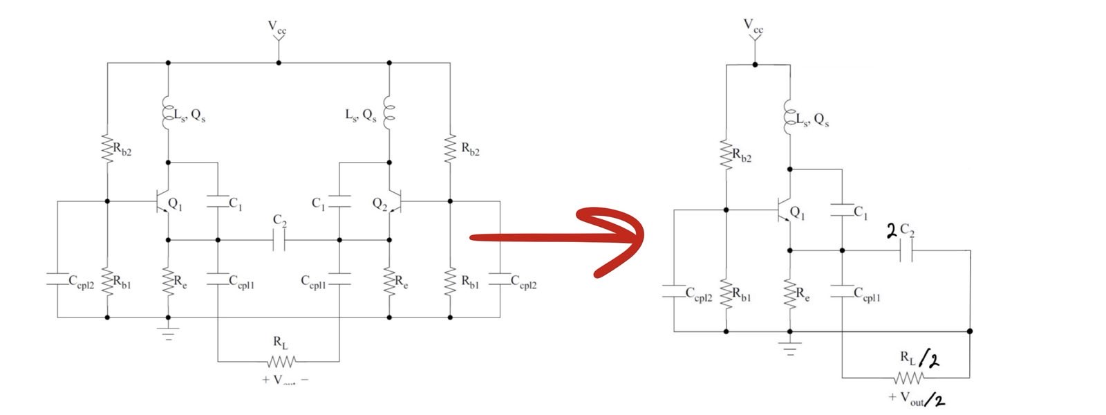

Design Considerations

Frequency Determination

Step one is converting the single ended Colpitts oscillator to small signal layout to find out where $C_A$ and $C_B$ sit.

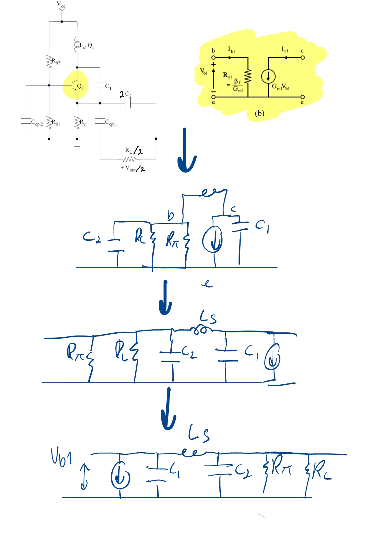
Comparing small signal model to Vitaliy Zhurbenko oscillator slides, the correct configeration is obvious, C_A is parallel to current source and $C_B$ is paralel to $R_L$:

Formulas relevant to small signal configeration

\begin{align} G_m=\frac{1}{R_b} \cdot \frac{C_a}{C_b} \end{align} \begin{align} \omega^2 = \frac{1}{L_c \cdot C_{ser}} \end{align}

\[\frac{G_m}{g_m(I_{EE})} = \frac{2\hat{I}_1(x)}{x\hat{I}(x)} \quad \left\{ \begin{aligned} x &= \frac{V_{b1}}{V_t} \\ g_m(I_{EE}) &= \frac{\alpha I_{EE}}{V_t} \end{aligned} \right.\]

Step 1: using Bessel fuctions find Gm/gm

\[\begin{aligned} x = \frac{V_{b1}}{V_t} &= \frac{0.5}{0.025} = 20 \Rightarrow \frac{G_m}{g_m} = 0.0975 \\ \text{As } \beta \text{ is large, } \alpha \text{ is assumed to be equal to 1.} \\ g_m &= \frac{I_{ee}}{0.025} \\ G_m &= 7.80 \text{ mS} \end{aligned}\]

Step 2: finding Resistive parasitics of transistor

\[R_{\pi} = \frac{\beta}{G_m} = 9404.89 \, \Omega\]

Then, $ R_b $ is computed using the parallel combination of $R_{\pi} $ and $ R_l $:

\[R_b = \frac{R_{\pi} \cdot R_l}{R_{\pi} + R_l} = 474.75 \, \Omega\]

Step 4: finally $C_a$ and $C_b$ can be calculated

\[\begin{aligned} \frac{1}{475} \cdot \frac{C_1}{C_2} &= 1.452\,\text{m} \\ (5.4\,\text{G} \cdot 2\pi)^2 &= \frac{1}{1.02\,\text{n} \cdot \frac{C_1 C_2}{C_1 + C_2}} \end{aligned} \quad \left\{ \begin{aligned} &C_1 = 3.216\,\text{pF} \approx 3 \text{pF} \\ &C_2 = 1.158\,\text{pF} \approx 1 \text{pF} \end{aligned} \right.\]

Decoupling Capacitors

To analytically determine the appropriate decoupling capacitors, two decoupling capacitors, ( C_{cpl2} ) and ( C_{cpl1} ), are used with the following requirements:

1. The reactance of ( C_{cpl2} ) and ( C_{cpl1} ) must satisfy:

   \[\frac{1}{\omega \cdot C_{cpl}} \ll R_L\]

   ensuring the capacitors are greater than ( 0.06 \, \text{pF} ).

2. For ( C_{cpl1} ), it must bypass ( R_E ), and its time constant, ( \tau_E = R_E \cdot C_{cpl1} ), should match the logarithmic decrement of the resonance circuit:

   \[\tau_E = \frac{2Q}{\omega} \quad \Rightarrow \quad C_{cpl1} = \frac{2Q}{\omega \cdot R_E}\]

Substituting the design parameters (( Q = 10 ), ( \omega = 2\pi \cdot 5.4 \cdot 10^9 )), the value of ( C_{cpl1} ) is:

\[C_{cpl1} = \frac{2 \cdot 10}{2\pi \cdot 5.4 \cdot 10^9} \approx 1.96 \, \text{pF}\]

The final selected values for ( C_{cpl2} ) and ( C_{cpl1} ) are 1 pF and 2 pF, respectively.

Decoupling Results

Before Adjustment

The initial design exhibited instability, leading to undesired oscillations.

---

After Adjustment

After refining the decoupling capacitors, the circuit achieved balanced stability, eliminating one sided oscilation.

Biasing

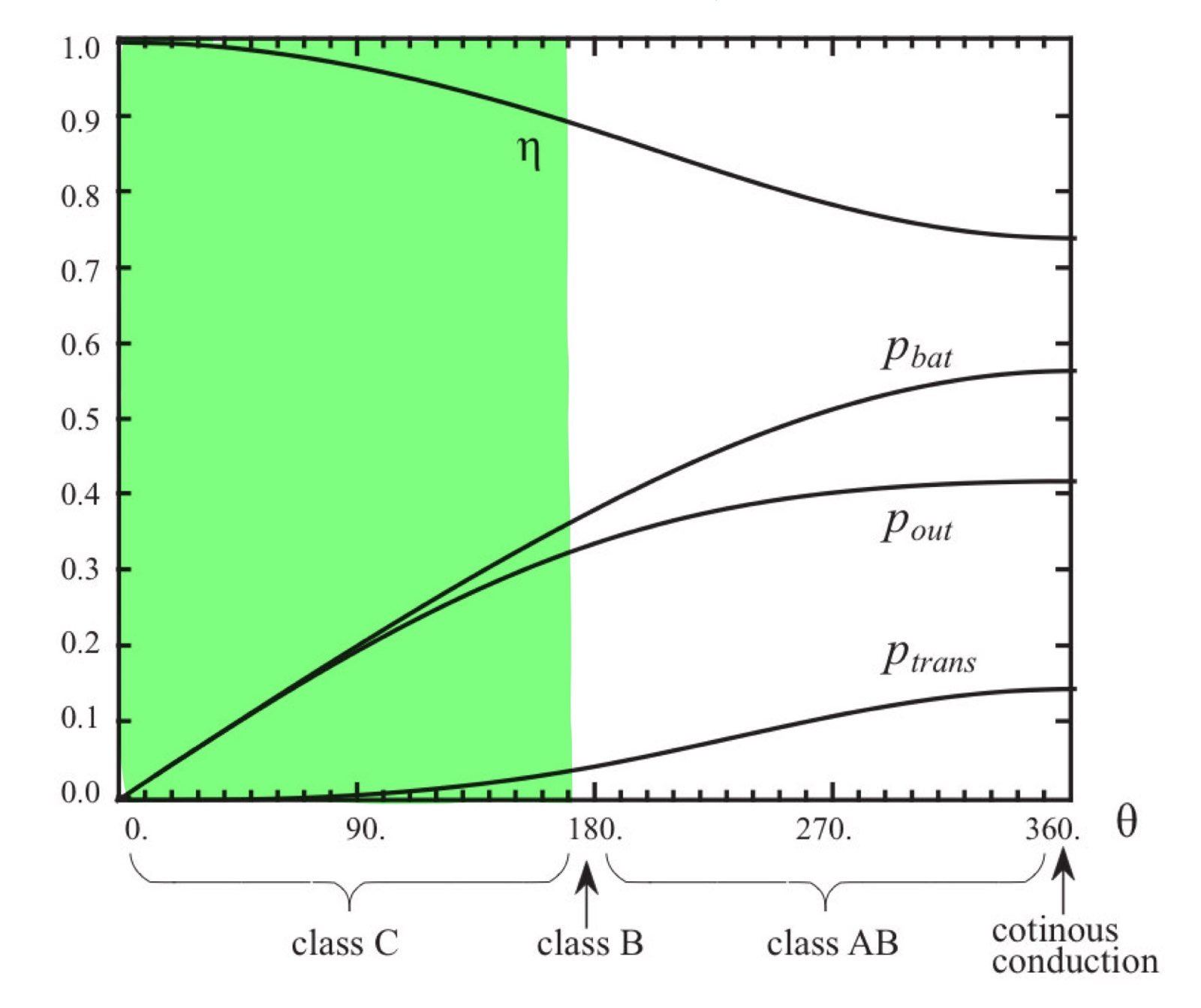A high-efficiency Class C biasing scheme was chosen to ensure minimal power consumption while maintaining stable oscillation. The selected biasing current was 5mA, which provided an optimal trade-off between gain and efficiency.

Using: \begin{align} R_e = \frac{V_{cc} - V_{ce}}{I_c(1 + \frac{1}{h_{FE}})}\end{align}

I determined R_e = 300Ω and R_1 = 1.7kΩ through analytical calculations and simulation verification.

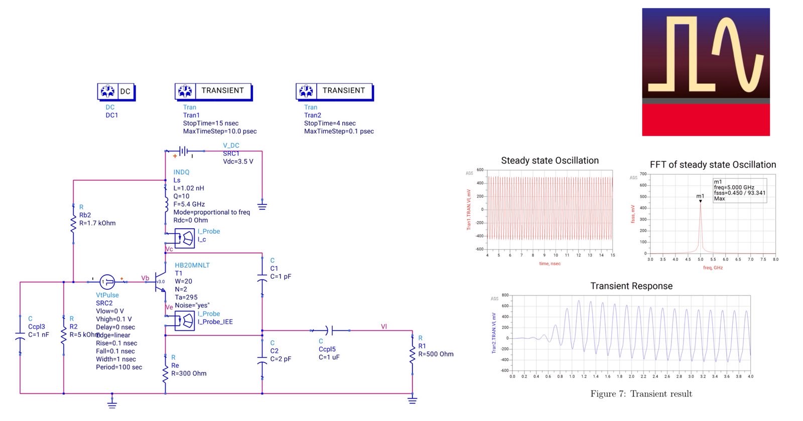
Simulation and Testing

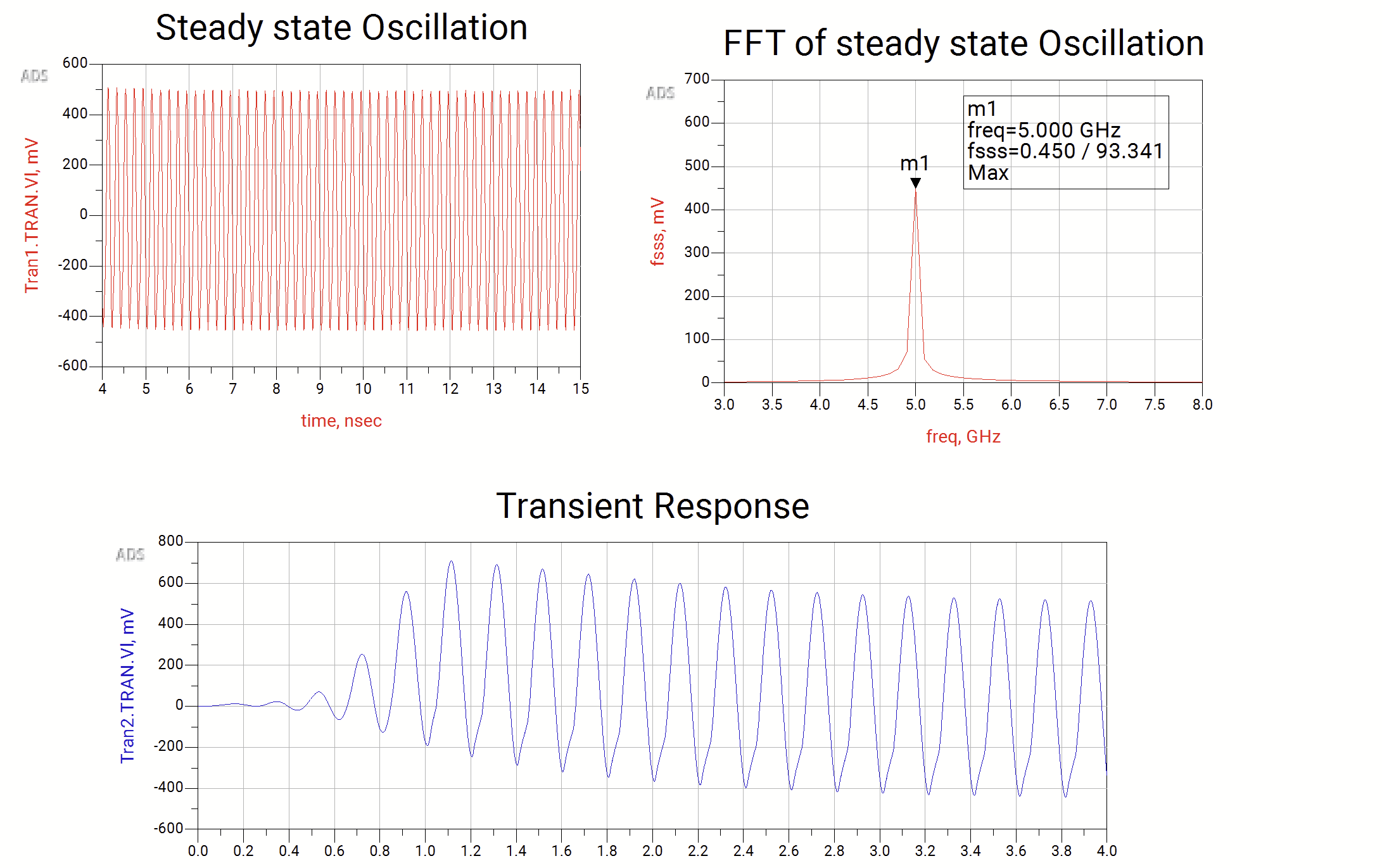
Transient Simulation

The design was simulated in Keysight ADS, verifying the following:

• Oscillation frequency: ~5GHz (slightly lower than the 5.4GHz target due to parasitics).
• Output voltage swing: 2Vpp, exceeding the minimum 1.5Vpp requirement.
• Stability: Rapid stabilization within 4ns.

Efficiency Analysis

Using Fourier analysis and Bessel functions, the conduction angle θ was found to be 95°, leading to an estimated efficiency >90%.

Conclusion

The 5.4GHz Colpitts oscillator achieved: ✅ Stable oscillation with low power consumption
✅ High output voltage (~2Vpp)
✅ Efficiency exceeding 90%
❌ Frequency needs further investigation

Minor frequency deviations were attributed to parasitic capacitances, suggesting future iterations could incorporate tuning capacitors for fine adjustments. This design successfully met its performance targets and demonstrated key RF design principles in practical implementation.